Java Regression Library - Linear Regression Model
07 Oct 2013Part 2 - Linear Regression Model
Welcome to part 2 of this tutorial series where we will be creating a Regression Analysis library in Java. In the last tutorial we covered a lot of theory about the foundations and applications of regression analysis. We finished off by coding up the RegressionModel abstract class, which will become the base of all our models in this library.
Prerequisites -
Make sure you have read and understand Part 1 of this tutorial series where I explained a lot of theory about regression analysis and regression models. I won’t be repeating much of the content so it’s a good idea to have a good understanding of it all before you read on with this tutorial.
Regression Library - Regression Models
In this tutorial we will be covering and implementing our first regression model - the simple linear regression model.
The Linear Regression Model
To start off with lets consider the first the Wikipedia article definition for the Simple Linear Regression Model:
Simple linear regression is the least squares estimator of a linear regression model with a single explanatory variable. In other words, simple linear regression fits a straight line through the set of n points in such a way that makes the sum of squared residuals of the model (that is, vertical distances between the points of the data set and the fitted line) as small as possible.
This is perhaps one of the easier to understand definitions. So in this model we have a single explanatory variable (X in our case) and we want to match a straight line through our points that that somehow ‘best fits’ all the points. in our data set.
This model uses a least squares estimator to find the straight line that best fits our data. So what does this mean? The least squares approach aims to find a line that makes the sum of the residuals as small as possible. So what are these residuals? The residuals are the vertical distances between our data points and our fitted line. If the best fit line passes through each of our data points, the sum of the residuals would be zero - meaning that we would find an exact fit for our data.
Consider this numerical example:
We have the data:
X         Y
2         21.05
3         23.51
4         24.23
5         27.71
6         30.86
8         45.85
10        52.12
11        55.98
We want to find a straight line that makes the sum of the residuals as small as possible. As it turns out the least squares estimator for this data set produces the straight line:
y = 4.1939x + 9.4763
as the line of best fit - that is, there exists no other straight line for which the sum of the residuals (the sum of the differences between the actual data and the modelled line) is smaller.
This makes a lot of sense as a line of best fit. There essentially exists no other straight line that could better follow our data set as that would mean the sum of the residuals would have to be smaller. So remember:
Residuals = the differences in the Y axis between the points of data in our data set and the fitted line from our model.

So in the linear regression model we want to use a least squares estimator that somehow finds a straight line that minimises the sum of the resulting residuals. The obvious question now is how can we find this straight line?
The Math
So we want to find a straight line that best fits our data set. To find this line we have to somehow find the best values of our unknown parameters so that the resulting straight line becomes our best fit. Our basic equation for a straight line is:
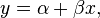
We want to find the values of a and ß that produce the final straight line that is the best fit for our data. So how do we find these variables?
Handily there is a nice formula for it (for those of us who don’t want to derive it):

Ok perhaps that formula isn’t that nice after all then at first glance. The good thing is it really isn’t all that bad when you get to know the symbols:
- x with a line over the top is called xbar = the mean of the
Xvalues in our data set - y with a line over the top is called xbar = the mean of the
Yvalues in our data set
The sigma (the symbol that looks like a capital E) is the sumnation operator. The good news for us programmers is that this symbol can be nicely converted into something we can all understand - the for loop - as we will see in a minute!
Now we could go off now and start trying to code up a solution to find ß, but it would be a lot easier if we could somehow modularise the formula a little more to make it easier to understand. Again handily the formula does that for us. Near the bottom is the formula we actually want:
Cov[x, y]
——————
Var[x]
Which stands for the covariance of x and y divided by the variance of x. Now we only have to find out those two calculations, divide them, and we have our result for ß.
We are only really worried about ß as finding a is easy once we have a value for ß. It’s just the mean of the y values minus the found value of ß multipled by the mean of the x values. Great!
Covariance and Variance methods
We first need to find out more about the covariance and variance functions and code up two small helper methods that we can then make a good use of in our linear model. Lets start with the covariance. I won’t be covering any of the theory about these functions as their is already a wealth of information out there for your to read on your own. We end up with another formula for the covariance of x and y:
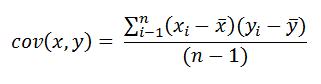
This one is a lot easier to understand. The only bit that requires attention is the sumnation on the top which as I said earlier can be roled out into a simple for loop! Under the sigma we have an i and at the top we have N (the size of our data set). Looking familiar already? We are essentially just looping from i = 0 to i = N. The idea is to just sum the result of the formula after the sumnation symbol for each time around the loop - using i along the way to access our data points (xi = x for example) - just like we do in a for loop to say sum the elements of an array!
It’s probably easier if I show the code and then explain it.
public static double covariance(double[] x, double[] y) {
 // Get the means of the x and y data first
 double xmean = mean(x);
 double ymean = mean(y);

    double result = 0;

    // loop through from i = 0 to the length of the data set (N in the formula)
    for (int i = 0; i < x.length; i++) {
        // Perform the calculation in the formula, adding each time to the result variable to get the final sum
        result += (x[i] - xmean) * (y[i] - ymean);
    }

    // Finally divide by the data set - 1 to get our final result
    result /= x.length - 1;

    return result;

}

// Calculate the mean of an array of data
public static double mean(double[] data) {
 double sum = 0;

    for (int i = 0; i < data.length; i++) {
        sum += data[i];
    }

    return sum / data.length;

}
It’s really all pretty self-explanatory for programmers. Everyone should be able to understand the mean method so I won’t cover that. In the covariance method we first get the means of each of our data points. This makes xbar and ybar in the formula. We then simply loop through our data set summing the results of the calculation:
(xi - xbar) * (yi - ybar). Hopefully you can see how this relates to the formula.
Thats it for the covariance method. Now onto the variance.
The formula for the variance is extremely simple if you understand the covariance. Again I won’t cover the theory behind the variance as there is already a lot of good information out there about it. The formula is:

The variance is also known as the sum of the squared deviations over the length of the data set, which can easily be seen by the formula. Again we have a simple sumnation that sums the differences between the data elements and the mean of the data set squared. We then divide this result by the length of the data set minus 1. Here is the code which makes use of the mean method from above:
public static double variance(double[] data) {
 // Get the mean of the data set
 double mean = mean(data);

    double sumOfSquaredDeviations = 0;

    // Loop through the data set
    for (int i = 0; i < data.length; i++) {
        // sum the difference between the data element and the mean squared
        sumOfSquaredDeviations += Math.pow(data[i] - mean, 2);
    }

    // Divide the sum by the length of the data set - 1 to get our result
    return sumOfSquaredDeviations / (data.length - 1);

}
I won’t explain this method as the comments do a good job. It’s really just a simple for loop that sums the result of a small calculation.
Coding up the linear model
Armed with a few helper methods for the covariance, variance and mean we can finally code up our linear model!
We first create a new class called LinearRegressionModel that inherits from our RegressionModel class:
public class LinearRegressionModel extends RegressionModel {

    // The y intercept of the straight line
    private double a;

    // The gradient of the line
    private double b;

    /**
    * Construct a new LinearRegressionModel with the supplied data set
    * @param x The x data points
    * @param y The y data points
    */
    public LinearRegressionModel(double[] x, double[] y) {
        super(x, y);
        a = b = 0;
    }

}
We have two private fields representing the coefficients of our fitted straight line. Now all we need to do is code up the overriden methods. First up is the .getCoefficients() method which returns an array containing the two coefficients:
/\*\*

-   Get the coefficents of the fitted straight line
-
-   @return An array of coefficients {intercept, gradient}
-
-   @see RegressionModel#getCoefficients()
    \*/
    @Override
    public double[] getCoefficients() {
     if (!computed)
     throw new IllegalStateException("Model has not yet computed");

        return new double[] { a, b };

    }
Then there is the evaluateAt(double) method which allows us to evaluate the fitted line at a certain point:
/\*\*

-   Evaluate the computed model at a certain point
-
-   @param x
-   The point to evaluate at
-   @return The value of the fitted straight line at the point x
-
-   @see RegressionModel#evaluateAt(double)
    \*/
    @Override
    public double evaluateAt(double x) {
     if (!computed)
     throw new IllegalStateException("Model has not yet computed");

        return a + b * x;

    }
Both methods are pretty easy. They both first check of the model has computed before returning a result. If not an exception is thrown. Now we only have to implement the compute() method to find the coefficients of our fitted line and we are done:
/\*\*

-   Compute the coefficients of a straight line the best fits the data set
-
-   @see RegressionModel#compute()
    \*/
    @Override
    public void compute() {

        // throws exception if regression can not be performed
        if (xValues.length < 2 | yValues.length < 2) {
            throw new IllegalArgumentException("Must have more than two values");
        }

        // get the value of the gradient using the formula b = cov[x,y] / var[x]
        b = MathUtils.covariance(xValues, yValues) / MathUtils.variance(xValues);

        // get the value of the y-intercept using the formula a = ybar + b * xbar
        a = MathUtils.mean(yValues) - b * MathUtils.mean(xValues);

        // set the computed flag to true after we have calculated the coefficients
        computed = true;

    }
Before we compute the values we must first check that both data sets have at least two values (refer to Part 1 for more details on why). If there are then we use the two formulas along with the helper methods (now inside a MathUtils class) to find the values of a and b that make up our line of best fit. It’s really not all that complicated when you separate it all out.
The Full Code
MathUtils:
/\*\*

-   Various helpful math functions for use throughout the library
    _/
    public class MathUtils {
    /\*\*
     _ Calculate the covariance of two sets of data
     \*
     _ @param x
     _ The first set of data
     _ @param y
     _ The second set of data
     _ @return The covariance of x and y
     _/
     public static double covariance(double[] x, double[] y) {
     double xmean = mean(x);
     double ymean = mean(y);

            double result = 0;

            for (int i = 0; i < x.length; i++) {
                result += (x[i] - xmean) * (y[i] - ymean);
            }

            result /= x.length - 1;

            return result;
        }

        /**
        * Calculate the mean of a data set
        *
        * @param data
        * The data set to calculate the mean of
        * @return The mean of the data set
        */
        public static double mean(double[] data) {
            double sum = 0;

            for (int i = 0; i < data.length; i++) {
                sum += data[i];
            }

            return sum / data.length;
        }

        /**
        * Calculate the variance of a data set
        *
        * @param data
        * The data set to calculate the variance of
        * @return The variance of the data set
        */
        public static double variance(double[] data) {
            // Get the mean of the data set
            double mean = mean(data);

            double sumOfSquaredDeviations = 0;

            // Loop through the data set
            for (int i = 0; i < data.length; i++) {
                // sum the difference between the data element and the mean squared
                sumOfSquaredDeviations += Math.pow(data[i] - mean, 2);
            }

            // Divide the sum by the length of the data set - 1 to get our result
            return sumOfSquaredDeviations / (data.length - 1);
        }

    }
LinerRegressionModel:
/\*\*

-   A RegressionModel that fits a straight line to a data set
    \*/
    public class LinearRegressionModel extends RegressionModel {

        // The y intercept of the straight line
        private double a;

        // The gradient of the line
        private double b;

        /**
        * Construct a new LinearRegressionModel with the supplied data set
        *
        * @param x
        * The x data points
        * @param y
        * The y data points
        */
        public LinearRegressionModel(double[] x, double[] y) {
            super(x, y);
            a = b = 0;
        }

        /**
        * Get the coefficents of the fitted straight line
        *
        * @return An array of coefficients {intercept, gradient}
        *
        * @see RegressionModel#getCoefficients()
        */
        @Override
        public double[] getCoefficients() {
            if (!computed)
                throw new IllegalStateException("Model has not yet computed");

            return new double[] { a, b };
        }

        /**
        * Compute the coefficients of a straight line the best fits the data set
        *
        * @see RegressionModel#compute()
        */
        @Override
        public void compute() {

        // throws exception if regression can not be performed
        if (xValues.length < 2 | yValues.length < 2) {
            throw new IllegalArgumentException("Must have more than two values");
        }

         // get the value of the gradient using the formula b = cov[x,y] / var[x]
         b = MathUtils.covariance(xValues, yValues) / MathUtils.variance(xValues);

         // get the value of the y-intercept using the formula a = ybar + b \* xbar
         a = MathUtils.mean(yValues) - b * MathUtils.mean(xValues);

          // set the computed flag to true after we have calculated the coefficients
          computed = true;
        }

        /**
        * Evaluate the computed model at a certain point
        *
        * @param x The point to evaluate at
        * @return The value of the fitted straight line at the point x
        * @see RegressionModel#evaluateAt(double)
        */
        @Override
        public double evaluateAt(double x) {
            if (!computed)
                throw new IllegalStateException("Model has not yet computed");
            return a + b * x;
        }

    }
Making sure it works
I will cover testing our Regression Library in depth in a later tutorial, but for now we will simply make sure that we get the same results as Microsoft Excel does for the same data set (from above).
public static void main(String[] args) {
 double[] x = { 2, 3, 4, 5, 6, 8, 10, 11 };

    double[] y = { 21.05, 23.51, 24.23, 27.71, 30.86, 45.85, 52.12, 55.98 };

    System.out.println("Expected output from Excel: y = 9.4763 + 4.1939x");

    RegressionModel model = new LinearRegressionModel(x, y);
    model.compute();
    double[] coefficients = model.getCoefficients();

    System.out.printf("Actual output from our code: y = %.4f + %.4fx", coefficients[0], coefficients[1]);

}
OUTPUT:
Expected output from Excel: y = 9.4763 + 4.1939x
Actual output from our code: y = 9.4763 + 4.1939x
Looks good to me!
That wraps up this tutorial where we implemented our first regression model. Be sure to check out the next tutorial where we cover the logarithmic and exponential models.
Thanks for reading!
Sources: Wikipedia